Diffusion Methods for Robotics
1 Overview
Generative models have been popular for many tasks in vision and language for several years. Since about 2015, diffusion models have become popular for image generation tasks like inpainting, superresolution, denoising, stylistic editing, relighting, text-to-image synthesis, and several other conditional image generation tasks. Their expressivity and ability to combine different concepts made them very popular over the previous generative methods such as Generative Adversarial Networks (GANs).
Diffusion models were soon employed for tasks in robotics such as trajectory generation, sub-goal generation, policy learning, etc due to these same characteristics of expressivity and compositionality. In this post, we’ll look at some background about simple diffusion models and how they are trained, their variants such as conditional models and latent-space models, and their use in robotics. We will discuss one specific use case in robotics, imitation policy learning, and look at a couple of papers in the space. Finally, we will discuss some areas of interest in the community today related to diffusion methods for robotics.
2 Background
This section will cover the background of what diffusion models are, how they work, and their use in conditional generation and latent-space generation.
2.1 Diffusion models
Diffusion models are a class of generative models inspired by non-equilibrium thermodynamics, introduced by 1. Just like any generative method, they try to model a data distribution and then sample new instances from that distribution. They initially became popular for image generation tasks like denoising, inpainting, super-resolution, editing, synthesis, etc but are now used for various tasks beyond image generation. Several interpretations and formulations of diffusion models have been proposed over the years (2, 3) but at the core, diffusion models consist of 3 major components: the forward diffusion process (to create a training dataset), the backward or reverse diffusion process, and a sampling procedure.
2.1.1 Forward diffusion process
Given a sample \(\mathbf{x}_0\) from some distribution \(q(\mathbf{x})\), the forward diffusion process iteratively adds small amounts of Gaussian noise to the sample in \(T\) timesteps to produce \(\mathbf{x}_1, \mathbf{x}_2, …, \mathbf{x}_T\).
As \(T \to \infty \), \(\mathbf{x}_T\) is equivalent to an isotropic Gaussian distribution. Formally,
where \(\beta_t\in(0, 1)_{t=1}^T\) is the variance schedule, which controls the amount of noise added at each step.
Given this, we can now run the forward process for all steps as \(q(\mathbf{x}_{1:T} \vert \mathbf{x}_0) = \prod_{t=1}^T q(\mathbf{x}_t \vert \mathbf{x}_{t-1})\)
Typically, \(\beta_1 < \beta_2 < ... < \beta_T\), i.e. the noise added is initially small and gets larger as we get closer to an isotropic Gaussian.
A reparametrization trick allows us to directly compute \(\mathbf{x}_t\) for an arbitrary time step \(t\) rather than sequentially, but I will skip that for the purpose of this post. We have now created noisy samples given a true sample from the distribution. The reverse process will aim to reverse this and learn the underlying data distribution while doing that.
2.1.2 Reverse diffusion process
The reverse diffusion process aims to learn \(q(\mathbf{x}_{t-1} \vert \mathbf{x}_{t})\) through a model \(p_{\theta}\) that aims to find the parameters \(\theta\) that maximise the sample probability, i.e., maximise the likelihood over \(n\) training samples. \[ \theta^* = argmax \prod_{i=1}^{n}p_{\theta}(\mathbf{x}^i) \]
We train a neural network to predict the distribution’s parameters (\(\boldsymbol{\mu}_{\theta}, \boldsymbol{\Sigma}_{\theta}\) such that \(p(\mathbf{x}_t) = \mathcal{N}(\mathcal{x}_{t-1}; \boldsymbol{\mu}_{\theta}, \boldsymbol{\Sigma}_{\theta})\) ). In practice, we learn to predict the noise, \(\epsilon_t(\mathbf{x}_t, t)\), at time \(t\) and use that to indirectly estimate \(\mathbf{x}_{t-1}\).
2.1.3 Sampling procedure
The simplest method of sampling is to simply follow the reverse process step-by-step and predict \(\mathbf{x}_{t-1}\) from \(\mathbf{x}_{t}\) for \(t \in \{T, T-1, ..., 1\}\). However, as you would imagine, this naive process can be very slow as \(T\) could range from a few tens to a few thousands of steps. Various methods (4, 5, 6) have been proposed to speed up sampling by using fewer sampling steps.
2.2 Variants
2.2.1 Conditional diffusion models
While unconditional generation is useful, most practical applications require conditioning the model on some input to control the output. For example, image tasks like inpainting, superresolution, etc take a noisy or degraded measurement of a sample and find a point on the true distribution that closely matches the input while also adhering to the data distribution.
There are two major types of conditional diffusion models, classifier-guided models and classifier-free guidance.
Classifier-guided diffusion models
Classifier-guided models (7) pre-train a separate classifier on the conditional task at hand. Then, the gradients of the classifier are incorporated into the noise prediction by the diffusion model. This flow of gradient causes the noise prediction to be consistent with the desired class prediction, thus resulting in a denoised sample that reduces the classifier loss. Further, the amount of classifier guidance (gradient) may be controlled by a hyperparameter, allowing for variability in the conditioning strength.
Classifier-free guidance
In classifier-free guidance (8), the diffusion model jointly learns a conditional and unconditional noise prediction. Here, the model is trained with paired data \((x_t, y)\) as well as unpaired data \((x_t, None)\). This training process allows the model to implicitly learn a classifier. At each timestep, the inputs to the noise prediction model are the current estimate, \(x_t\), the current timestep, \(t\), and the conditioning variable, \(y\).
2.2.2 Latent-space diffusion models
Diffusion models were initially developed for images, so they operate in the image or pixel space. However, 9 introduced latent space diffusion models where rather than denoising and predicting the data directly, you predict some latent embedding of the data. This latent embedding is typically learnt but can be any representation. This allows us to model high-dimensional data by representing it in a lower dimensional latent space, making both training and inference much faster.
3 Diffusion Models in Robotics
While diffusion models have mainly been applied to image generation and other generative modeling tasks, recent work has shown promising applications in robotics tasks such as with imitation learning and reinforcement learning. They have also been used for image/video diffusion where the model generates realistic long-horizon video or image frames. Given expert trajectory data, diffusion models have been used to generate trajectories by interpolation and extrapolation of paths, constraints, etc.
Diffusion models offer several useful properties in the context of robotics, including:
- Expressiveness: They can learn arbitrarily complicated data-distributions
- Training stability: They are easy to train, especially in contrast to GANs
- Multimodality: Ability to handle multimodal data and generate diverse outputs
- Compositionality: Capacity to incorporate constraints and guidance during the generation process
For applications such as policy learning via imitation learning, we often think of the data being represented by diffusion models as states, actions, or latent embeddings and not necessarily images or videos. Remember, diffusion models are only learning to model some data distribution and the kind of data is immaterial. We therefore “diffuse” over states, actions, or latent embeddings.
While diffusion models have been used in various robotics tasks as mentioned above, we will focus on using diffusion models for imitation learning and dive deeper into it.
3.1 Diffusion Methods for Imitation Policy Learning
Simple imitation learning, such as vanilla behavior cloning, takes a series of states and their corresponding expert actions to learn a policy that would imitate the expert. While this simple method is often quite effective, it suffers from OOD (Out-Of-Distribution) states during inference for which a policy was never learnt, and the inability to do any long-horizon planning.
Improvements have been proposed to mitigate the data distribution problem, such as DAgger (10) where an expert is queried on-demand to provide demonstrations when an OOD state is encountered (Interactive Imitation Learning), and Inverse Reinforcement Learning (IRL) techniques where we learn a reward function from the expert demonstration data which is then used to train a policy. In GAIL(11), they use a GAN-like setup where a generator (policy network/actor) generates action trajectories and an adversary classifies these trajectories as coming from the expert or the generator. To deal with longer-horizon planning, methods such as ACT (12) have been proposed that predict a series of actions (trajectories) from a state or a history of states.
Several improvements of the above ideas have been proposed over the years but recently, diffusion models have become a popular choice for solving these problems of OOD data, long-horizon planning, training stability, sample efficiency, etc.
Policy learning with diffusion models has been done by conditioning these models on some context, either in the form of embedded states or observations(13, 14), vision (15, 16, 17) or vision and language, and the output of these models could be intended next state(s), actions(s) or subgoal(s) in the form of pose, actuations, images, language, etc. We will discuss the ideas from two papers that aim to use different inputs/outputs to learn a policy either directly or indirectly.
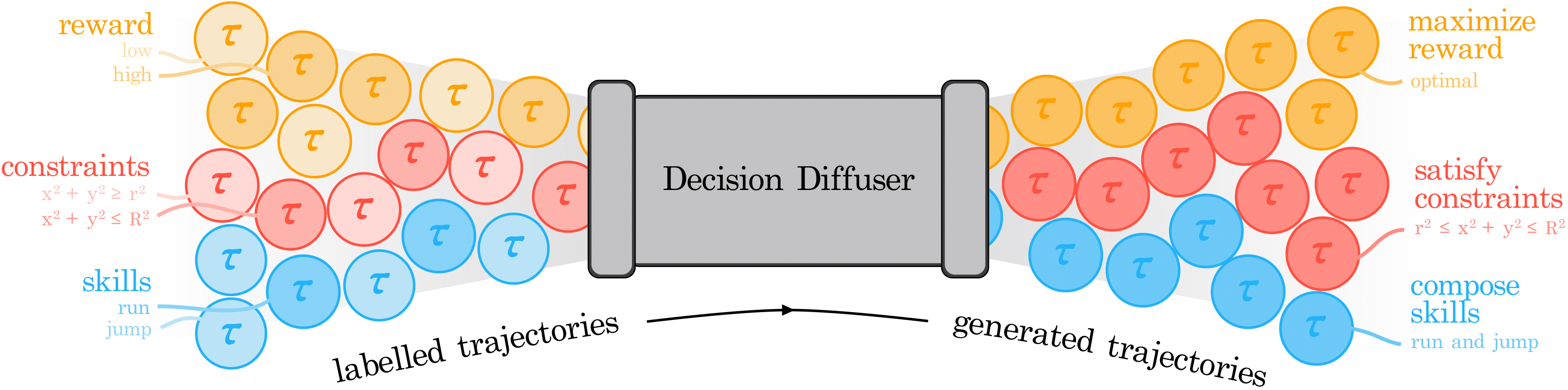
Is Conditional Generative Modeling all you need for Decision-Making? [Ajay et al. (2022)]
This paper introduces using a conditional diffusion model, DecisionDiffuser, for sequential decision making (SDM) where the model learns the trajectory distribution, conditioned on some variable. They use sub-optimal expert trajectories and show that their model can combine the best parts of the training trajectories to generate new trajectories that maximise some objective. They show 3 types of conditioning, (1) on the return of the trajectory to maximise returns, (2) on an encoding of the constraints to satisfy a combination of constraints in the environment, and (3) an encoding of the skills being used in a trajectory to compose skills.
They show results on 3 tasks for these 3 types of conditioning. For maximising returns, they compare against offline RL methods on a variety of tasks in simulation and show that their model is comparable to or outperforms offline RL methods. For constraint satisfaction, they show generation of trajectories to stack or rearrange blocks given constraints on their relative positions. For skill composition, they train a quadroped robot’s gait on trajectories with different gaits such as bounding, pacing, or trotting individually and show the generation of trajectories with multiple gaits composed together.
It is worth noting here that the output of the model is a trajectory of states and not directly a policy. They then use a reverse dynamics model to get actions from states. They also use a trajectory of states encoded in some way as input, and we will now look at some work where they directly use images to represent the state.
NoMaD: Goal Masked Diffusion Policies for Navigation and Exploration [Ajay et al. (2023)]
NoMaD showed the use of diffusion models to directly learn a policy (action trajectory) from image data. They model the state as the set of RGB images from the last \(t\) timesteps and allow optionally conditioning on a goal image. They use a vision transformer to encode the state and goal into a context vector, which is used for conditioning the diffusion model. The diffusion model outputs a set of candidates of a series of \(k\) future actions.
They train the end-to-end model on 2 large datasets of 100+ hours of real-world video data. They split their training dataset to mask the goal image 50% of the time, which allows them to learn a policy for both directed and undirected navigation. They show their policy outperforms several baselines for goal-direction navigation and exploration in 6 real-world unseen environments. This work shows the possibility of having a single end-to-end diffusion based model for long-horizon planning. Here, they directly learn a policy (trajectory of actions) from image observations.
5 Discussion of current research directions
Given the advances in language and vision-language models, multimodal models for robot policy generation is a popular topic: combining vision and language for long-horizon planning tasks with mult-step processes. Several recent papers use language and vision models to generate sub-goals, which are then converted to action trajectories using diffusion models.
Several other works have been aimed at creating an end-to-end large scale multi-modal foundation model for robotics. Octo (18) is one such recent work that uses very large-scale robotics data to create a generalist manipulation model given visual, language, or other multi-sensory data. They use a large transformer model with diffusion heads for generating actions. The direction today seems to be aimed at creating a generalist multi-modal foundation model (with transformers and diffusion models), similar to what OpenAI’s GPT models did for language.
Further, computational efficiency for training and inference of diffusion models is relatively low, meaning we need faster training and efficient sampling mechanisms to enable real-time generation. When diffusing over high-dimensional spaces such as image or video, this becomes particularly important. Another problem arises from the need for large amounts of training data. Many models have been trained on large-scale simulation data since that is easier to acquire, but we need good Sim2Real transfer models or sample efficient models that are able to learn similarly complex distributions with less real-world data.
6 Conclusion
Diffusion models are a powerful class of generative models, that offer advantages over previous methods such as GANs with improved generalizability, more stable training while learning complex distributions, flexibility to handle multi-modal data, and compositional ability. They also work exceptionally well for long-horizon planning for robotics tasks.
These advantages make them very useful in robotics where complex distributions must be estimated from few samples or sub-optimal samples. The papers discussed above show that we can learn optimal trajectories or combine skills/constraints from different training trajectories while training with sub-optimal single skill/constraint data.
However, due to the sampling process of diffusion models, they are often slow to run inference on and thus pose a challenge when dealing with high dimensional data or real-time inference. Especially in the case of robotics where compute and time are often limited, we need more efficient sampling mechanisms and ways to speed up inference. The field of diffusion models is relatively new, and their use in robotics is even more recent. In the last few years, we have seen the literature on diffusion models for robotics grow rapidly, and they are likely to continue to be a valuable tool for roboticists for many years.
7 References
Articles
- https://lilianweng.github.io/posts/2021-07-11-diffusion-models/
- https://github.com/mbreuss/diffusion-literature-for-robotics
Paper references
-
Deep Unsupervised Learning using Nonequilibrium Thermodynamics ↩
-
Generative Modeling by Estimating Gradients of the Data Distribution ↩
-
Progressive Distillation for Fast Sampling of Diffusion Models ↩
-
High-Resolution Image Synthesis with Latent Diffusion Models ↩
-
A Reduction of Imitation Learning and Structured Prediction to No-Regret Online Learning ↩
-
Learning Fine-Grained Bimanual Manipulation with Low-Cost Hardware ↩
-
Is Conditional Generative Modeling all you need for Decision-Making? ↩
-
Goal-Conditioned Imitation Learning using Score-based Diffusion Policies ↩
-
Diffusion Policy: Visuomotor Policy Learning via Action Diffusion ↩
-
NoMaD: Goal Masked Diffusion Policies for Navigation and Exploration ↩