In my first year as an undergrad CS student, I was fascinated by a lot of things. Evolutionary or genetic algorithms was one such fascination that lasted long enough for me to write a system that evolves to reach a goal. In this post, I’m going to explain the idea behind applying Darwin’s theory of evolution to solve optimization problems and am going to show that we can visualize how they work.

This post is for:

1. People who are fascinated by genetic algorithms and want to get started with using them
2. People who have no idea what genetic algorithms do but think it sounds interesting
3. Anyone else who loves learning new stuff :)

We will write a system to visualize how evolution can be applied to a simple optimization problem. The goal will be to find the fastest path between two points while avoiding obstacles.

Those of you who already know the basics of genetic algorithms and wish to skip ahead to the implementation can go here.

What is evolution?

According to wikipedia,

Evolution is change in the heritable characteristics of biological populations over successive generations. These characteristics are the expressions of genes that are passed on from parent to offspring during reproduction. Different characteristics tend to exist within any given population as a result of mutation, genetic recombination and other sources of genetic variation.

It’s alright if you don’t understand all the words in this definition but I assume it is broadly understood. But how do these concepts apply to computational problems? What is a gene or the concept of reproduction in our world of computational problems?

I’m going to explain a little about the biological concepts to understand the motivation and then move on to the computational equivalents of things. Don’t worry about the biology terms if you’ve not heard of those before.

Gene

In biology, a gene is a sequence of neucleotides (Adenine,Thymine, Guanine, Cytosine or ATGC). An organism has many such genes that determine it’s characteristics. In humans, we have genes that determine our skin and hair color, height and other physical characteristics. We’ll use an organism’s gene to store how it behaves in our simulated world.

Reproduction and Genetic Recombination

When organisms mate, their genetic material is combined to form the genetic material of the offspring. The way this combination takes place determines the characteristics of the offspring. This combination may lead to characteristics in the offspring that aren’t directly observable in either of the parents, but are expected based on the rules of genetic recombination.

Mutation

Every now and then, the combination of the genetic material during reproduction is imperfect; the offspring’s gene may contain sequences that are not a result of mating but of a random alteration. This is rare and usually does not affect the characteristics of the organism too much. We will use this as a tool to give the system enough randomness to recover from local optima - more on this later.

Why Would Evolution Work For Optimization?

The infinite monkey theorem states that a monkey hitting keys at random on a typewriter keyboard for an infinite amount of time will almost surely type any given text, such as the complete works of William Shakespeare.

Now while this may sound ridiculous, it is theoretically true (proof). Although, this would take longer than the age of the known universe (~13.8 billion years < infinite time).

Even if the monkey gets one word right using this approach, that effort is useless if it is followed by gibberish. The monkey would need to get entire sentences and paragraphs right for us to solve the problem at hand. It would be useful if we could somehow store the successful efforts of the monkey from the past.

Assume that the genetic information of the monkey determines the sequence of words it types. The idea here is to task an entire population of monkeys with writing shakespeare’s works and select those monkeys that are typing more sense. We then breed these selected monkeys to form the next generation with the goal that the next generation will be closer to being able to solve the problem.

With each new generation, the monkeys would have more and more favourable characteristics and we’d finally solve the problem. Although it’s not so simple in reality and there are nuances that make this hard, the motivation for applying evolution to this problem, and any optimization in general could be understood this way.

Our Genetic Algorithm - The implementation

I will assume that readers have basic knowledge of Python, or any other programming language. A lot of the code will be pseudo-code that you will have to implement yourself in your favorite language so knowledge of a specific languge is not essential. I’ve intentionally kept the code to a minimum so that you figure out how to make it work yourself.

I will share my complete Python code at the end if someone is stuck and needs to look through it.

Part 1 (Problem formulation)

We’ll be building a system where a population has one simple goal: To travel from a fixed birth point to another fixed target point in the smallest possible time while avoiding obstacles.

For this implementation, we will be using a 3-dimensional system where the birth point, target and obstacles are 3-dimensional objects in .

From the above description, we can see that we need to define atleast 3 things:

1. Organism along with it’s gene and fitness
2. The target
3. The obstacles

Organism

The organism has at least the following properties:

1. Position - A vector in
2. Velocity - A vector in
3. Fitness - How well it has performed
4. Alive flag - Whether it is alive
5. Success - Whether it succeeded in accomplishing the goal and how long it took
6. Gene - Something that determies how it behaves. We will discuss this in more detail

class Organism:
    vec3 position;
    vec3 velocity;
    float fitness;
    bool alive;
    int success;
    list[Force] gene;

class Force:
    float magnitude;
    vec3 direction;

The vec3 class is a helper class I’ve written with basic functionality for dealing with 3-dimensional vectors. You can find the complete Python code for that class here but I suggest writing it yourself and enriching it as and when you need more functionality.

Target

The target is simply a point, disc or sphere in space. In our case, it is a sphere.

Obstacles

For simplicity, I’ve allowed for only cuboidal obstacles. However, you can choose any shape and topology as long as you’re able to implement the collisions/interactions with the organisms.

Organism genes and fitness

We need to come up with a gene that is able to capture all the necessary information to determine the organisms behaviour in our simulation. For this, lets construct the gene to contain a force that the organism applies at each timestep to move itself in its environment (you could think of it as a force that will to be applied to the organism by us, the simulator, to make the organism move). Since we run the simulation for a certain period of time, we can apply these forces throughout that duration. The gene is therefore a list of forces.

As the organism interacts with its environment, it accrues either positive or negative points. Since we want the organism to reach the target and avoid obstacles, we will reward organims (give positive points) for getting close to the target and penalize them (give negative points) for colliding with the obstacles. We also want to make them reach the target fast and hence we also factor in the time while giving points. Further, we want them to remain in a fixed boundary and hence penalize organims that stray out of the box.

So to sum up, our fitness criteria looks something like this:

And the pseudo-code looks something like this:

for each organism o:
    if not o.alive:
        do nothing and continue

    o.fitness = 1
    o.fitness /= o.closest_record_dist_to_target
    o.fitness /= hit_time if success else current_iteration

    # Reward for hitting target
    if dist_to_target < target_radius:
        o.success = current_iteration
        o.fitness *= 10e4
        o.alive = False

    # Penalize for hitting obstacles or walls
    for obstacle in self.obstacles:
        if o.position is in boundary of obstacle:
            o.alive = False
            o.fitness *= 10e-4
    if o.position is not in boundary of container:
        o.alive = False
        o.fitness *= 10e-4

You could keep adding more conditions and experimenting with how the process of evolution takes place with different fitness criteria. A suggested exercise is to try to modify the fitness function such that it also encourages organisms to stay at or near the target after they hit it and not move away.

The fitness function is probably the most important part of the whole process since it is the basis for selection and creation of the next generation. Tweaking this function can drastically change the results.

Part 2 (Simulation)

Now that we have some structure to the problem, we can begin to think about the process of evolution that we want to simulate and how we can achieve that. The first thing to notice is that we need to define a population and define the rules for evolution in that population.

Initial population

The initial population would consist of organisms with random gene sequences. What this means is that they will move around randomly, with most of the population perishing by colliding with obstacles or the walls of the container.

The initial population is a list of organisms with the following properties:

position = birth_point
velocity = vec3(0, 0, 0)
fitness = 1
alive = True
success = -1
gene = [Force(random_float, random_vec3) for _ in duration_of_simulation]

Moving the organisms

Since we encoded the movement of organisms in the gene, we use the gene to determine the motion at each timestep of the simulation. The update is done using the Euler integration method (basically the method to calculate position and velocity based on the force applied) and that looks something like this:

for each organism o:
    force = o.gene[current_iteration]
    o.velocity += force.magnitude * force.direction.normalize()
    o.position += o.velocity

Evolution

The major steps involved in simulating the evolution are selection and mating.

Selection

This is the process of selecting organisms of the species that are the fittest (in terms of whatever fitness function we have defined). There are various theories of selection but we will proceed with the simplest - The top N organisms that have highest fitness, as defined by our fitness function, will be selected to form the mating pool.

We will, however, implement this idea indirectly through something called Roulette Wheel Selection. Think of a roulette from a casino. When you spin the roulette, the chance of the ball landing in each of the pockets is the same. Now if 60% of the wheel’s pockets were black and 40% red, the probability of the ball landing in a red pocket becomes 0.4. Roulette wheel selection does something similar by allocating pockets to organisms in proportion to their fitness values. We then spin the wheel as many times as required to pick organisms for mating in the next step.

# Roulette wheel selection
# Higher fitness will mean more of the same organism is added to the mating pool.
# This is a way to give a higher mating probability to higher fitness

mating_pool = []

for o in population:
    normalized_fitness = o.fitness/max_fitness_in_population
    normalized_fitness *= 1000  # Arbitrary multiplier

    for i in range(int(normalized_fitness)):
        mating_pool.append(o)

Mating

Now that we have mating pool, we can begin to randomly pick 2 organisms to mate (Randomly already accounts for the probablities since we added pockets in proportion to fitness). We repeat this process as many times as we need to create the desired population size for the next generation of the species.

1. Genetic recombination

Once we pick 2 organisms, the mom and dad, we need to define the method used for genetic recombination or crossover. I’ve used a simple and effective single point crossover mechanism but I encourage you to experiment with others.

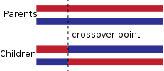
As shown above, you pick a random point in the length of the gene and splice the first segment of the mother with the second segment of the father to create the first child. You can similarly create the second child too.

2. Mutation

Suppose the first generation of the species happened to only move towards the obstacles or that the species is performing decently well and is staying alive but no one is reaching the target. Here even the fittest individuals in the population show no promise of ever reaching the target. Are we stuck in a local optimum? How can we overcome this?

You may notice that the above method of recombination only utilizes the present generations’ fittest individuals’ knowledge but what if the entire population of the present generation is clueless? To get over this, we need to have inquisitive children who think out of the box and don’t necessarily follow in their parents’ footsteps.

This is done by adding some randomness to the next generation (many biological species also rely on random mutation for genetic diversity in their populations). This ensures that the species does not get stuck in a local optimum. Just like with crossover, there are multiple mutation types but we’ll stick to a simple one - Replace the force in certain positions of the gene with random forces. These positions are randomly selected based on a parameter called the mutation rate. Smaller the mutation rate, lower the number of positions replaced and vice-versa.

for index in gene.length:
    if random.uniform(0, 1) < mutation_rate:
        gene[index] = Force(random_float, random_vec3)

Performing the simulation

With all the discussion above on selection and mating, you are now equipped with everything you need to write the simulation. I assume the steps in problem formulation (organism-gene and fitness, target, obstacles) have already been implemented. To summarize, the steps for simulation are as follows:

- Create the initial population
- For each generation in the simulation:
   - For each timestep/iteration of the generation:
     - Update position and velocity of all organisms
     - Calculate fitness for all organisms
   - Perform selection to prepare the mating pool
   - Mate the organisms in the mating pool using the principles of crossover and mutation
   - Reset the population. For each organism set:
     - position = birth point
     - velocity = vec3(0, 0, 0)
     - alive = True
     - success = -1

If you are stuck, you can find the complete Python implementation here

Part 3 (Visualization of simulation)

Once we have set up the above simulation, we have only the species’ fitness to indicate how the system is performing. Without visual proof of the process, it seems incomplete. Now we will try to visualize the simulation we have just set up.

Since this section is very dependent on implementation, I will be sharing most of my code as I walk through the process. You can choose to skip this section or just skim through it if you’d like to implement it yourself.

I am using PyGame as the framework for visualization, which you can learn how to download and install here. Since our simulation works in and pygame doesn’t support 3D graphics, I’m going to be visualizing the world as a 2D orthographic projection of the actual 3D world. Don’t worry if this sounds daunting right now. I promise it’ll get clear once we start coding. If you’re wondering why I didn’t just pick a framework that supports 3D graphics, the idea of this post is to familiarize you with genetic algorithms and introducing the complexitities of 3D graphics is an unnecessary overhead that I wished to avoid.

Lets dive straight in.

Simulation class

We create a simulation class to encapsulate everything related to a single simulation - population, mutation rate, target, obstacles, etc.

class Simulation:
    def __init__(self, population_size, duration, generations, mutation_rate):
        self.population_size = population_size
        self.duration = duration
        self.generations = generations
        self.mutation_rate = mutation_rate

        self.organisms = []
        self.mating_pool = []

        self.birth_position = vec3(800, 850, 0)
        self.target = vec3(800, 100, 200)
        self.target_radius = 20
        self.obstacles = [Box(vec3(500, 500, -600), vec3(1100, 400, 600))]
        self.container = Box(vec3(0, 0, -800), vec3(1600, 900, 800))

        self.avg_fitness = []

We’ve used a Box class to define an obstacle. It looks something like this:

class Box:
    def __init__(self, p1, p2):
        self.p1 = p1
        self.p2 = p2

        self.rectangles = [
            Rectangle(
                vec3(p1.x, p2.y, p1.z),
                vec3(p2.x, p1.y, p1.z)
            ),

            Rectangle(
                vec3(p1.x, p2.y, p2.z),
                vec3(p1.x, p1.y, p1.z)
            ),

            Rectangle(
                vec3(p1.x, p1.y, p1.z),
                vec3(p2.x, p1.y, p2.z)
            ),

            Rectangle(
                vec3(p1.x, p2.y, p2.z),
                vec3(p2.x, p1.y, p2.z)
            ),

            Rectangle(
                vec3(p2.x, p2.y, p2.z),
                vec3(p2.x, p1.y, p1.z)
            ),

            Rectangle(
                vec3(p1.x, p2.y, p1.z),
                vec3(p2.x, p2.y, p2.z)
            )
        ]

    def isInBox(self, p):
        if p.x < min(self.p1.x, self.p2.x) or p.x > max(self.p1.x, self.p2.x):
            return False
        if p.y < min(self.p1.y, self.p2.y) or p.y > max(self.p1.y, self.p2.y):
            return False
        if p.z < min(self.p1.z, self.p2.z) or p.z > max(self.p1.z, self.p2.z):
            return False
        return True


class Rectangle:
    def __init__(self, p1, p2):
        self.p1 = p1
        self.p2 = p2

Then we need to initialize pygame and create an empty window. This process should be done only once and in the beginning.

def initDrawing(self):
    pygame.init()
    self.screen = pygame.display.set_mode([1600, 900])

Once we have the screen object reference, we can use it to draw other stuff in the window. We now need to write a function to draw the organisms, obstacles and target for each iteration of each generation. As you recall, the environment is in but we will visualize it in . Hence we need to define an orthographic projection for all these objects. That essentially boils down to finding an orthographic projection for a single point.

To define this, we need to first define the plane on which we are going to project the point. One simple way to define a plane is by specifying a point on the plane and the normal to the plane. Take some time to think about how this works and that for a given point and normal, only one possible plane could exist.

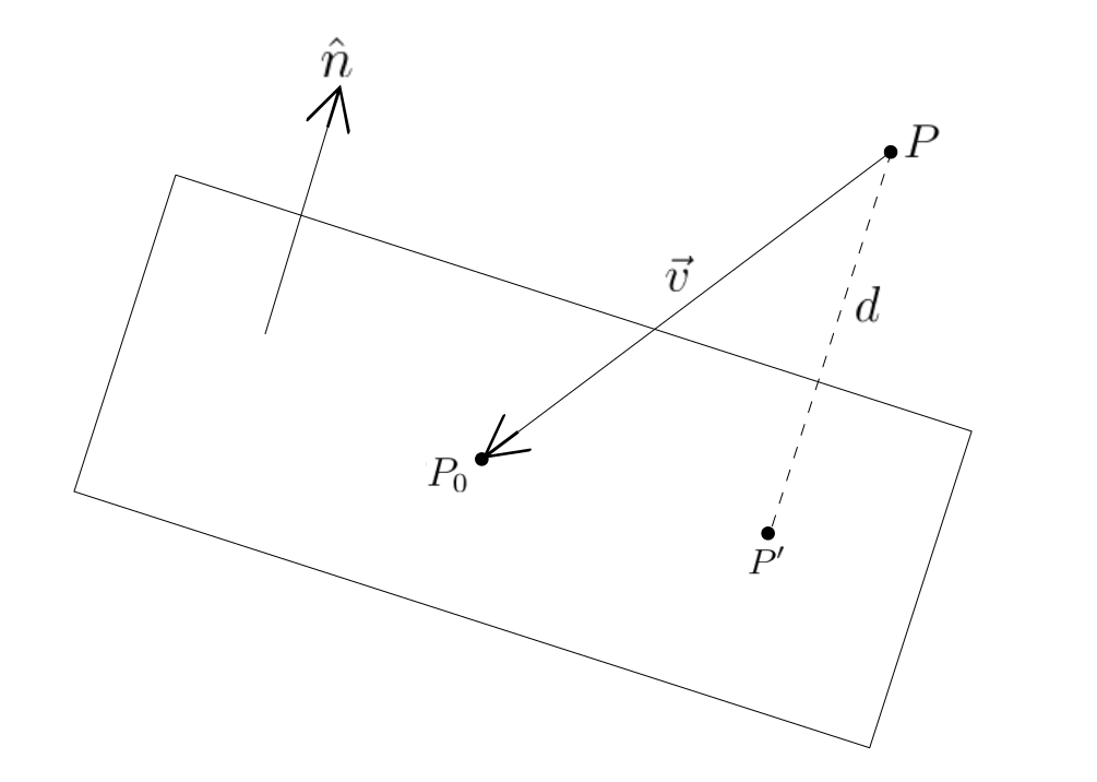
In the image above, is a point on the plane and is the unit normal vector to the plane. Point needs to be projected on this plane defined by and . Consider the vector . The perpendicular distance can be calculated as and the projection of the vector on is . The projected point is then . To sum up,

def project3D_on_2D(point3D, n, p):
    v = point3D-p
    perp_dist = fabs(v.dot(n))
    projected = point3D-perp_dist*n
    x = int(projected.x)
    y = int(projected.y)
    return vec3(x, y, 0)  # or just use projected if no integer casting

We then also define how the obstacles look in 2D. Since we have only cuboidal obstacles defined by rectangles, we’ll add similar projection logic to the Rectangle and Obstacle classes.

# Rectangle class
def get2D(self, n, p):
    p1 = project3D_on_2D(self.p1, n, p)
    p2 = project3D_on_2D(self.p2, n, p)
    return (p1.x, p1.y, fabs(p2.x-p1.x), fabs(p2.y-p1.y))

# Box class
def get2DRectangles(self, n, p):
    return [rect.get2D(n, p) for rect in self.rectangles]

Now we can go ahead and write the function to draw all our elements on the screen.

def draw_organisms(self, iter):

    # Provides an orthographic projection
    n = vec3(0, 0, 1)  # Normal to the x-y plane
    p = vec3(0, 0, 0)  # Any point on the plane

    self.screen.fill((255, 255, 255))
    # Draw target
    target_2D = project3D_on_2D(self.target, n, p)
    target_2D = (target_2D.x, target_2D.y)

    pygame.draw.circle(self.screen, (0, 0, 0), target_2D, 20)
    pygame.draw.circle(self.screen, (0, 255, 0), target_2D, 15)
    pygame.draw.circle(self.screen, (255, 0, 0), target_2D, 10)

    # Draw obstacles
    for o in self.obstacles:
        rects = o.get2DRectangles(n, p)
        for r in rects:
            pygame.draw.rect(self.screen, (100, 100, 100), r)

    # Draw organisms
    for o in self.organisms:
        color = (0, 0, 0)
        if not o.alive:
            if o.success > 0:
                color = (0, 255, 0)
            else:
                continue  # Don't draw dead organisms
        pos = project3D_on_2D(np.array(o.position), n, p)
        pygame.draw.circle(self.screen, color, (pos.x, pos.y), 5)

    # Replaces the buffer with the screen. This is a mechanism to render without stutter or artefacts
    pygame.display.flip()

If you’ve done everything right, the end result should look similar to this:

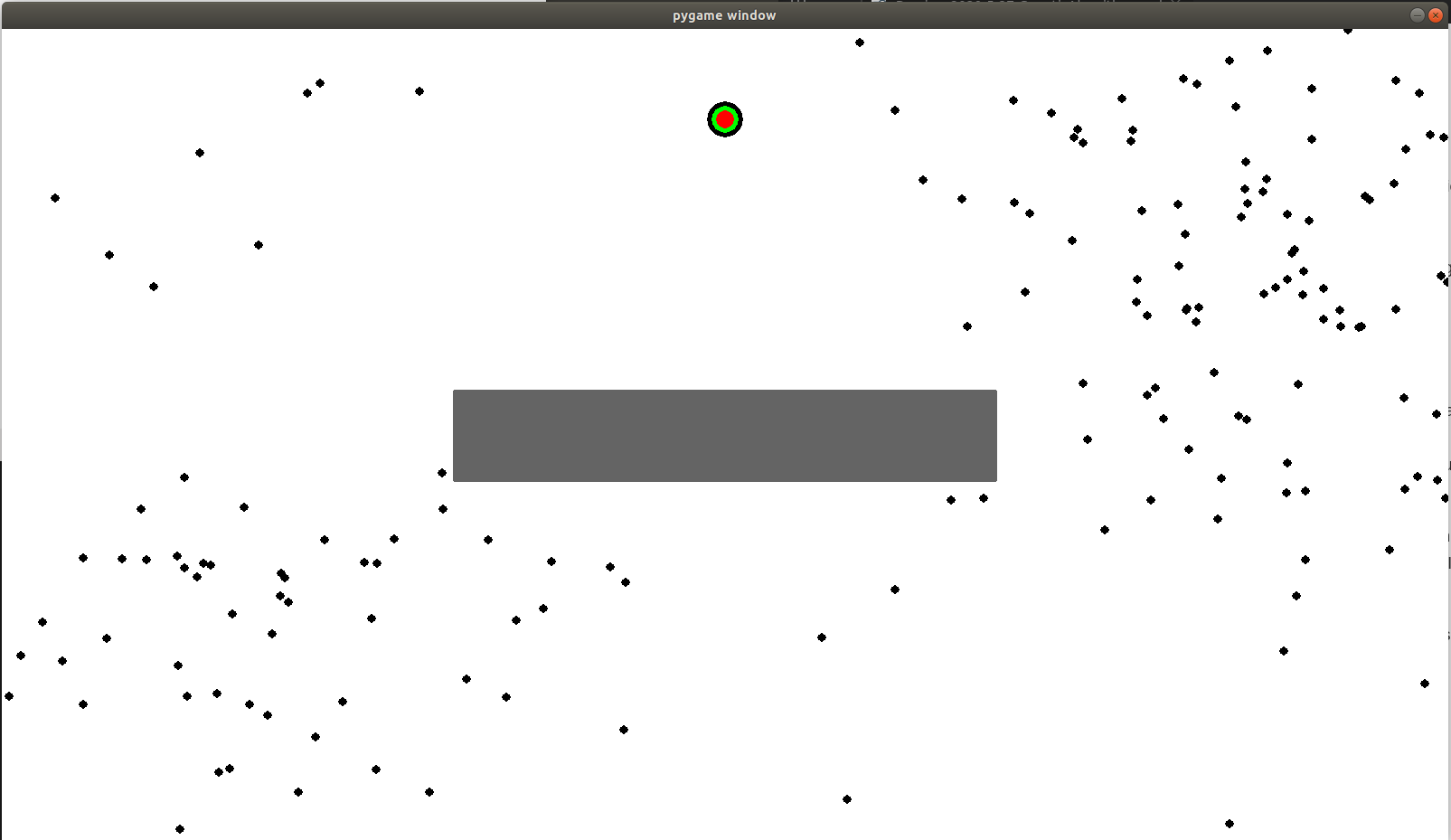
If you’re stuck, you can look at the complete code here.

Part 4 (Results)

If you let the simulation run for a while, you kind of get an idea about how the system is performing. You can subjectively tell whether the process is working or not. However, we want to quantify the progress and objectively say how well the system is performing. For this, one simple way to understand the species’ performance on the whole is to take the average fitness per generation and plot it on a graph.

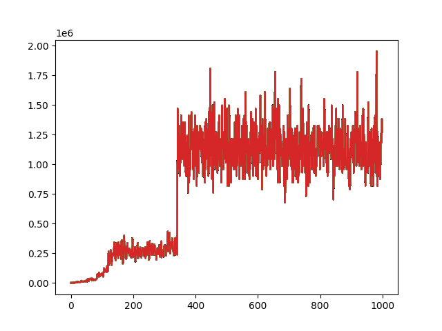
Here, the x-axis represents the generation and the y-axis represents average fitness of the population. The absolute fitness numbers don’t mean that much but notice how the values change and then flatten after a point. This happens when the system reaches the best local optimum point it could find. I’m still calling it local and not global since we can’t prove that it is optimum in this case. It could be both - either a good local optimum or the global optimum.

Notice how the system was stuck in a local optimum for ~200 generations (150 to 350). It was finally able to break through due to the process of mutation. This is possible even now and we could possibly find a better solution if we kept running the simulation.

What next?

As you probably realize, this is an extremely simplified tutorial. There are numerous methods of selection, mutation, ways to introduce genetic variation, processes like gene flow, genetic drift, etc. that you could learn.

This problem was intentionally chosen for this introduction as it can easily be solved in a few generations with simple techniques. Try increasing the number of obstacles or changing their topology and the challenges will become apparent. Genetic algorithms are considered excellent for solving certain types of optimization problems but for others, they are impractical.

If you’re interested, I suggest trying to apply genetic algorithms to any arbitrary optimization problem, preferably one you have previously solved using other methods and see how it compares. Can you find the right fitness function to make the system generate satisfactory results. If not, is there a mathematical limitation?

I suggest taking a look at this very interesting project where an AI has been written using genetic algorithms that can autonomously write code - AI Programmer: Autonomously Creating Software Programs Using Genetic Algorithms. Here is a good tutorial for this project.